A Chow test is used to check for a structural change between two regressions:
- The null hypothesis H0 is that all coefficients in the two regressions are the same.
- The alternative hypothesis H1 is that at least one of the coefficients is different.
The standard Chow test is joint, checking all coefficients together. However, more often we care about whether an individual coefficient is equal across two groups. If that’s our purpose, we wouldn’t really use the standard Chow test, or state in our work that “we use the Chow test to check the equality of the coefficient on X across the two subsamples”.
In this post, I first show how to perform the standard Chow test. Then I show how to perform a test checking if an individual coefficient is equal across two groups.
Perform the standard Chow test
Assume that we have two groups of observations. We have stacked (combined vertically) the two groups and generated a variable group, which takes the value of either 1 or 2, to indicate if an observation belongs to either group 1 or 2.
We perform the following regressions on the two groups separately:
y = a1 + b1*x1 + c1*x2 + u for group == 1
y = a2 + b2*x1 + c2*x2 + u for group == 2
It’s important to note that the standard Chow test is used to test whether the assertion a1==a2, b1==b2, and c1==c2 holds true jointly; it cannot be used to test whether any single one of them holds true.
The commands for the standard Chow test are listed below:
ge g2=(group==2)
regress y c.x1##i.g2 c.x2##i.g2
test 1.g2 1.g2#c.x1 1.g2#c.x2
The last command is equivalent to:
contrast g2 g2#c.x1 g2#c.x2, overall
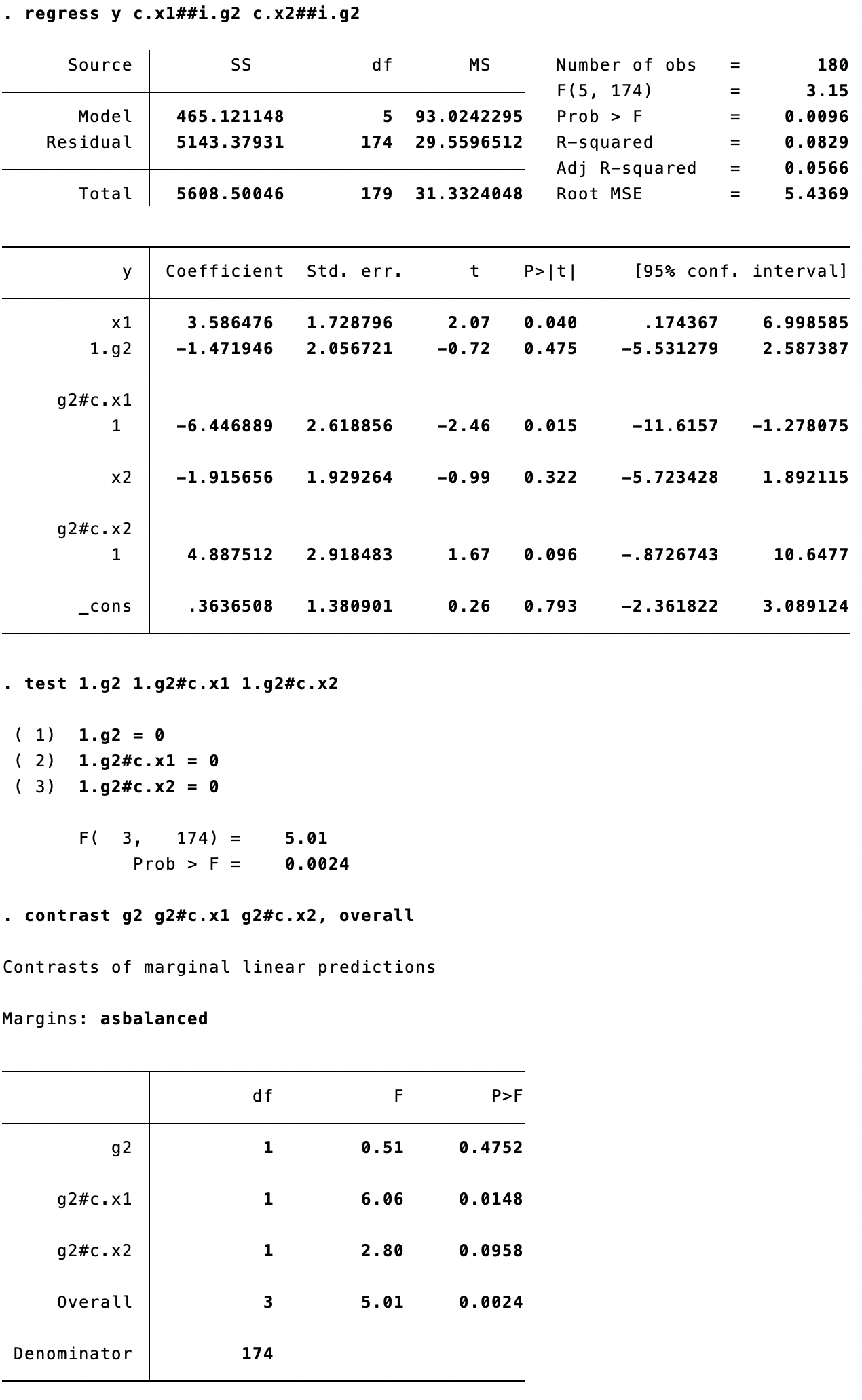
The test command and the contrast command (see the line of “Overall”) report the same results. Please note: (1) the F-stat for each independent variable is the square of the corresponding t-stat reported in the regression result table; (2) unlike the z- and t-distributions, the F-distribution is strictly nonnegative and has only a right-tail rejection region. In other words, the F-test is equivalent to a two-sided t-test and cannot be transformed to a one-tailed test.
Test the equality of individual coefficients
More commonly, we’d like to test whether a1 == a2 across the two groups (or b1 == b2). If the equality of an individual coefficient is our main interest, we should set up a pooled regression with the group indicator interacting with every independent variable.
Fortunately, under the hood of the standard Chow test is the pooled regression we have to resort to. We only need to check the regression result table presented above:
- If we want to test if a1 == b1, then check the t-stat on
1.g2#c.x1 - If we want to test if b1 == b2, then check the t-stat on
1.g2#c.x2
Both one-tailed (if the null hypothesis is directional, such as a1 <= a2) and two-tailed (if the null hypothesis is non-directional, such as a1 == a2) tests are possible.
Another option to perform the test is to use the following commands:
regress y x1 x2 if group==1
est store coefa
regress y x1 x2 if group==2
est store coefb
suest coefa coefb
lincom [coefa_mean]x1-[coefb_mean]x1
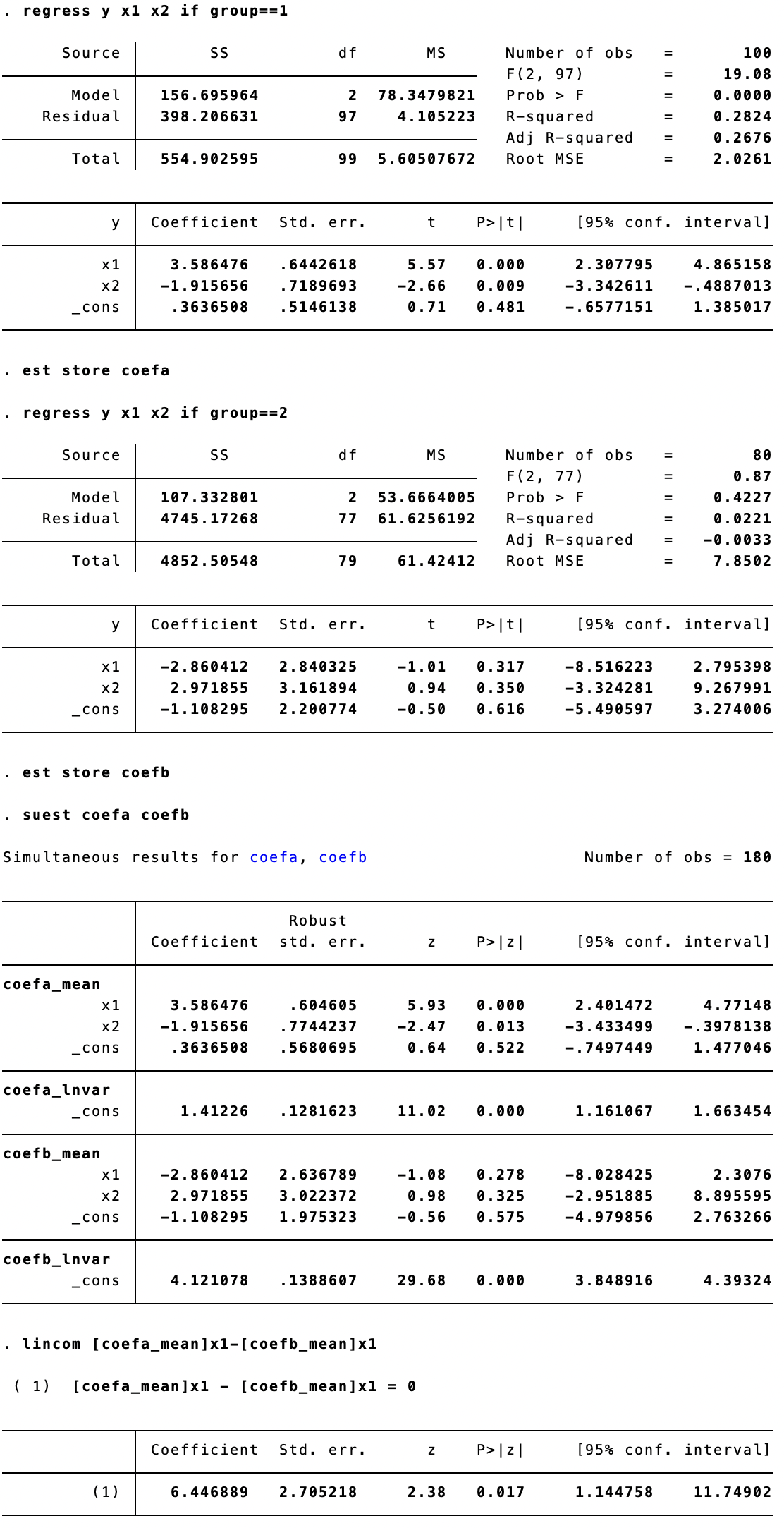
The benefit of this set of commands is that the difference in coefficients is reported directly, and the z-stat allows a one-tailed test as well.
I benefit from the two useful articles from Stata’s official website:
Can you explain Chow tests?
How can I compute the Chow test statistic?